LIBS
Inspection
NDT

How to EvaluateAccuracy
and Why You Should Calculate the Error Margin of Spectroscopy Measurements
We must be able to estimate the error in a spectroscopy measurement to assure ourselves, and our customers, of the true composition of the material.
By Marty Schreck
As international quality standards become increasingly demanding, you need to be confident in your QC analysis results – whether you are using an XRF, LIBS or OES analyzer. Without an accurate error margin, you simply cannot be sure that your parts meet specifications.
Whichever analysis method you use, every measurement made has an error margin associated with it. Usually, we try to reduce the error margin by using the best and most appropriate measurement system. For example, to measure a small component, we would use a micrometer and not a meter rule. Yet while the error margin can be reduced, it is never eliminated.
Once we accept that the error always exists, we can see that the statement such as ‘the Cr content is 20%’ is incomplete. We need to add an error margin to be sure that our component will meet the specification.
Another thing to watch out for is when the measurement value appears accurate because it has a lot of significant figures: i.e. the material carbon content is 0.13345%. There is still a level of uncertainty, even if the value is to five decimal places.
In spectroscopy, we measure because it is essential that our products have the right composition and hence quality. Therefore, we must be able to estimate the error in a spectroscopy measurement to assure ourselves, and our customers, of the true composition of the material.
Different Types of Error
Gross errors
A gross error would result in a measurement lying completely outside a ‘green area’ and would probably be picked up as an anomaly. Process errors, such as sample contamination during preparation, can cause gross errors as can defective samples, such as cavities in the measurement area, or running the incorrect measurement routine. Gross errors can be avoided through training and adhering to correct procedures.
Systematic errors
Systematic errors usually relate to trueness and give a consistent offset between the mean of the measured sample and the expected result. These are due to equipment faults, such as a lack of maintenance, worn parts or poor calibration. As the offset is consistent for every measurement within a defined area of interest, it’s possible to measure the offset and then incorporate a correction factor into your sample measurements.
Random errors
Random errors relate to precision. The greater the random variation, the less precise the measurement and the larger the error margin. Unlike systematic errors, they are unpredictable and are estimated with statistical methods. These measurement fluctuations can be due to inhomogeneity of the sample, tiny changes in the measurement environment and the measurement uncertainty of the reference samples used for calibration.
The goal is to increase precision as much as possible with good procedures and well-maintained equipment. Systematic errors can be determined by a straightforward calculation, whereas random errors follow a statistical model.
Introduction of Statistics
Random errors obey statistical laws, which is good news for us because we can apply basic statistical analysis to predict them. Let’s say that we have measured the height of every woman in America. If we plotted a graph of number of people against height, the graph would look like this.
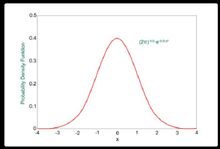
Image 1: Gaussian curve
There would be more women of average height near the center, and fewer at the tall and short end of the spectrum. This distribution of results is called a normal distribution. This normal distribution tells us that our measurement system follows predictable patterns of behavior and gives us the most important value in estimating the error margin of our measurements – the standard deviation.
Standard deviation (denoted by σ) is a numerical value that tells us by how much the typical (standard) results differ (or deviate) from the mean value. In other words, it tells us how spread out the results are.
Going back to our women’s height example. If our mean value is 170cm, and we have determined a value for σ of 2 cm, then we can say with confidence that 68.25% of women in America will be 170 cm +/- 2 cm tall, and 95.45% of women will be 170 cm +/- 4 cm tall.
For our application in spectroscopy, the smaller the value of standard deviation, the narrower the distribution curve and the more precise our measurements.
In reality, we do not usually measure a large enough sample size to accurately calculate σ for an entire population. We might just measure the height of women in single town for example. In this case, we say the standard deviation is ‘estimated’ and use the symbol ’s’.
Trueness Accuracy of the Mean
Accuracy is how near our measured value is to the expected value. The level of accuracy is dependent upon two factors:
Precision. The repeatability of measured values. If I measure the same sample several times, at the same point with the same equipment running the same procedure, how repeatable are my results?
Trueness. If I take several measurements, does the mean value match the expected value? This is also called the ‘accuracy of the mean’.
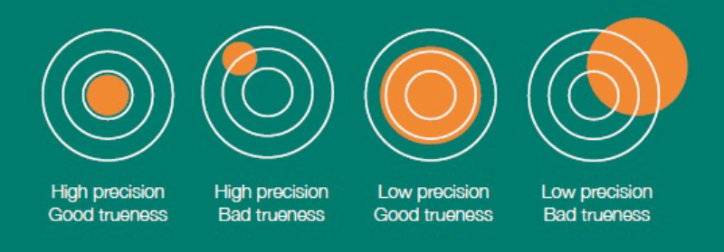
It is possible to have good precision, yet poor trueness. And it is possible to have high trueness (accuracy of the mean) and poor precision. For a truly accurate result, we want both high precision and trueness.
Fundamentally, spectroscopy is a comparative analysis method. We calibrate our instruments using standard reference samples and the instrument uses the results of these measurements to calculate a quantitative composition of an unknown sample.
This is why the first step in measuring anything is to calibrate the instrument within the desired measurement range.
However, despite our best efforts, sometimes our readings deviate from the expected value. This is seen when we take a certified reference sample with a known composition and measure it in our own instrument. We may see a difference in the measured mean from the expected value.
Regression analysis minimizes this divergence between the certified value and the measured value of the certified sample. However, you may still see residuals – deviations between reading values and certified values after regression analysis.
Ultimately, with a regression analysis of a large number of samples, the residuals will show the systematic deviation in the readings, i.e. the offset of the average of the mean from the expected value. And we can use this information to calculate the error due to the systematic deviation of the mean.
Calculation of Total Measurement Uncertainty
The ability to accurately estimate the total measurement uncertainty is so important that the regulatory bodies ISO and BIPM (Bureau International des Poids et Mesures) both give recommendations for ascertaining measurement uncertainty. Their guidelines are known as GUM: Guide to the Expression of Uncertainty in Measurement.
Why Calculate Measurement Uncertainty?
Routinely calculating the confidence interval or error margin in your spectroscopy measurements means you have to adopt certain extra practices in your operations. For example, you will have to take several measurements of each part instead of one. You will have to become familiar with the right form of statistical analysis and then find a way (or choose software) that will make the right calculations every time you make a measurement. So, why is it so important to calculate the margin of error in spectroscopy?
Firstly, without an accurate error margin, you simply cannot be sure that your parts meet specification as we have mentioned before. Whether gauging composition or measuring thickness, out of spec parts may result in rework, scrap, in-field failure and potential reputational damage. If you have accurately determined the margin of error for your components, you can see more easily if they are likely to be out of specification before they cause problems for your customers.
Secondly, internationally recognized quality management systems (QMS) include measurement system analyses (MSA). This means you cannot become certified for some international quality standards unless you have a robust MSA in place; and that will include a calculation of the measurement uncertainty for your spectroscopy measurements. For example, the IATF 19649 standard is the automotive industry’s most widespread standard for quality. The standard is designed to be implemented in conjunction with ISO 9001, and a clause in section 7 of IATF19649 deals exclusively with measurement system analysis. If you are selling into the automotive industry, or one like it that demands high quality standards, you will find that a robust measurement system analysis procedure that includes measurement uncertainty is essential.
We should point out that once the procedures are adopted into your operations, they become second nature. Once set up correctly, most spectroscopy instruments have the capability to carry out the statistical analysis calculations for you.
Conclusion
There is no such thing as an error-free measurement. Here is what to remember in your quest to search for the true value:
- Individual measurements are not complete if they do not include a measurement uncertainty or error margin.
- Multiple measurements are mandatory to gain the relevant statistical information.
- For spectroscopy, we must first calibrate the instrument in our region of interest before the analyzer can measure quantitively. Systematic errors (accuracy of the mean) can only be determined by measuring samples of known composition. This has a knock-on effect that we can only state confidence levels for defined areas of interest.
- If you take a reading and it is not what you expected, you must consider the uncertainty of your measurement. This must take into account precision (confidence intervals) and trueness (systematic deviations from the expected mean).
If you would like to find out more about this topic, visit hhtas.com/search-for-true-values to download a free detailed guide on how to obtain true values.
Image source: Hitachi High-Tech Analytical Science
Ian R. Lazarus is president and CEO of Creato Performance Solutions, providing leadership development, training, and solutions to support operational excellence.
Marty Schreck, applications manager for the Americas, Hitachi High-Tech Analytical Science.
Jim L. Smith has more than 45 years of industry experience in operations, engineering, research & development and quality management.

Febraury 2022 | Volume 61 | Number 2